What you will learn:
- Create a New Spreadsheet
- Add or Delete Columns and Rows
- Freeze a Row
- Coloring Selected Fields
- Add, Subtract, Multiply, and Divide Across Multiple Cells
- Multiply and Divide
1) Go to your Gmail inbox and open Google Drive (or go to drive.google.com).

2) Click on the “Drive” icon.

3) Click on “Create” and “Spreadsheet.”
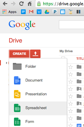
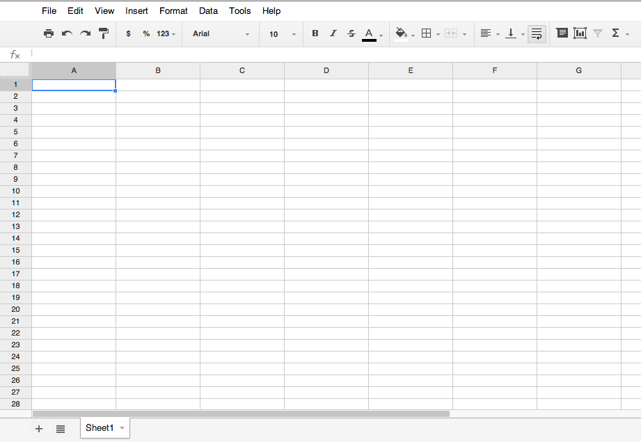
4) You will open a blank spreadsheet.
Add or Delete Columns and Rows
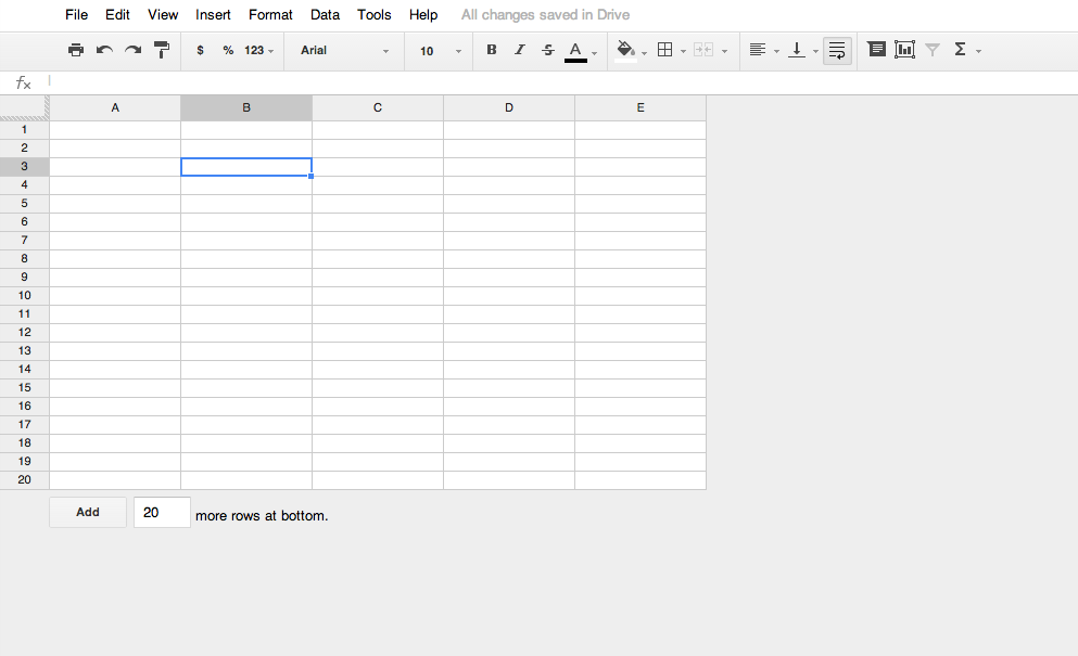
1) The following steps will describe how to add or delete columns. The image below will be the resulting finished template.
2) Let’s examine the difference between rows and columns. A column is the name given to vertically stacked cells, while a row describes a horizontal cross-section of cells.
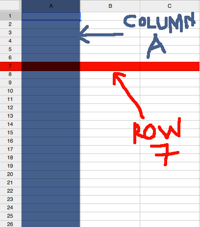
3) To delete unnecessary cells within a spreadsheet, you must first make a selection. If you are following along with this tutorial, click on a cell under column E. Scroll to the end of the spreadsheet, hold Shift, and click on another cell in the same row but under column T.
4) Click on Edit>Delete columns E-T.
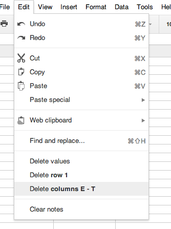
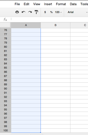
5) Alternatively, try deleting some cells within a vertical stack. Click on cell 21 under column A. Hold Shift and scroll down to row 100. Click cell 100 under column A, causing a selection that should look like the image below.
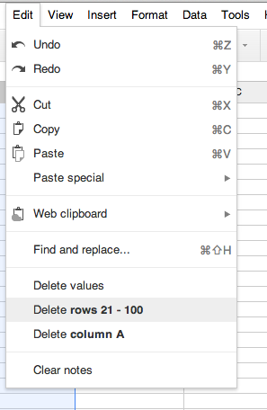
6) Click on Edit>Delete rows 21-100.
Freezing a Row
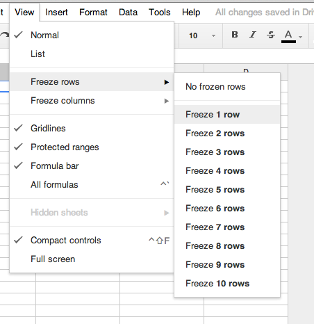
1) In order to freeze a row, click any cell as shown in the image below. This technique is effective for long spreadsheets because it allows you to create labels for categories that will always remain visible, regardless of scrolling.
2) Click View>Freeze rows>Freeze 1 row.
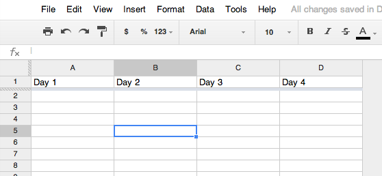
3) The row is now frozen, so you can fill it with whatever categories you want. In the example, I froze two rows and labeled the days of the week alongside the items to be tracked each day.
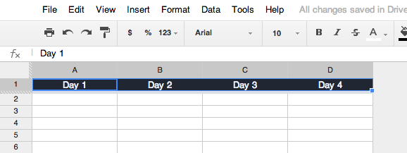
4) This example uses a four-day work week as the format. To follow along, type “Day 1”, “Day 2”, “Day 3”, and “Day 4” in a single frozen row across the top.
5) To center the labels in the middle of the columns, first Shift+Select all of the occupied cells in the frozen row.
6) Now, click the format drop-down in the menu and select the center align icon.
Coloring Selected Fields
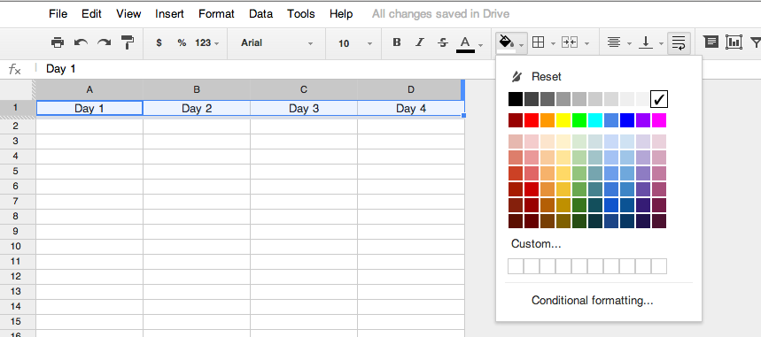
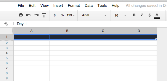
1) Select the cells within the row or column that you want to color. For this example, I have selected the frozen row at the top of my spreadsheet. In order for these labels to stand out, I will be filling the field with black and changing the text color to white.
2) Click the paint bucket to bring up this swatch field. Select black.
3) If the last step was successful, the cell should appear completely black. You will not be able to see the text until you change the font color.
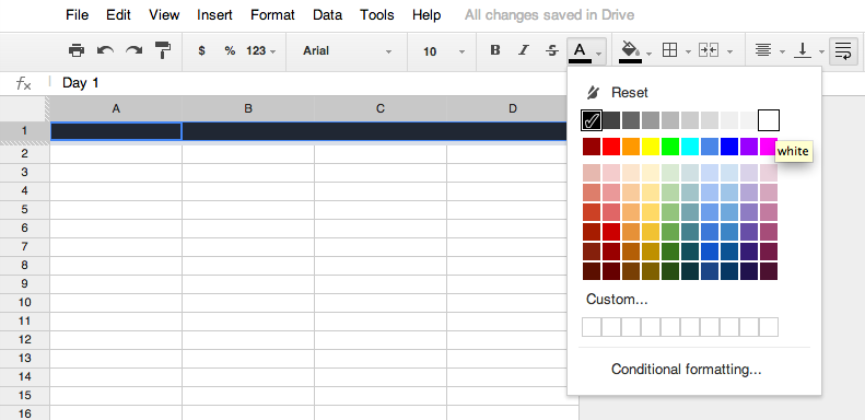
4) To do so, click the “A” symbol with the line below it and select the color white. Your words should now appear.
Magic!
Add, Subtract, Multiply, and Divide Across Multiple Cells
1) Now for the fun stuff: MATH!
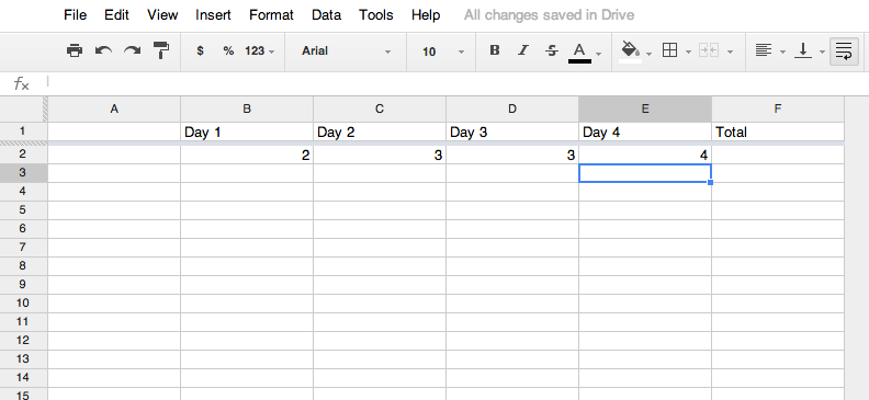
Let’s start with the basics. Below each day, enter some numbers. For the purposes of the example, these numbers correspond to the comic pages that you’ve produced within a given period.
On Day 1, I made two pages. Day 2 meant three more pages, and so on. You can enter the same numbers, but any numbers will do.

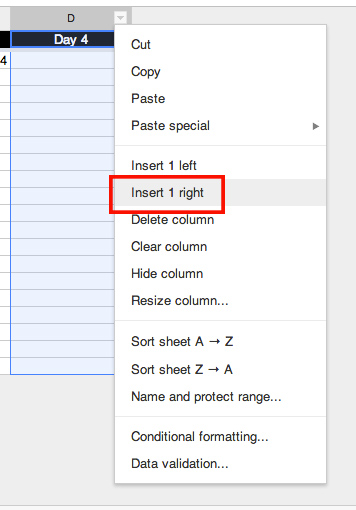
2) The next step will require two additional columns. To add a column, click the letter at the head of a column directly next to where you want the new column to appear. For our purposes, click column D. A drop-down menu will appear. Click “Insert 1 right”.
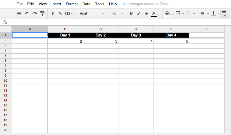
3) Add another column to the left of column A by repeating the last step. Click column A, but click “Insert 1 left” instead. Your spreadsheet should now look like the image below.
4) Enter titles for the new columns in the frozen row at the top of the spreadsheet. The left column should say “Weeks” and the right column should say “Totals.” Match both the cell color as well as the text color, and center the text.
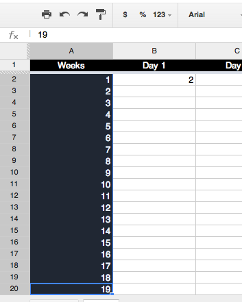
5) Below column A, label the rows from one to nineteen and change both the field and text colors.
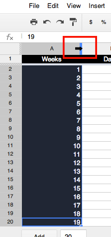
6) To resize the column, click towards the top of the cell that says “A” until you see an arrow key appear. You can now drag the column to resize it.
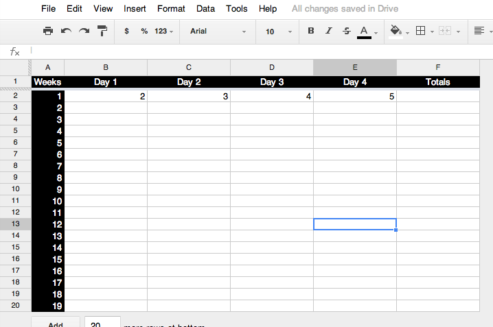
7) Your spreadsheet should look like the image below.
8) Now for the math part. Click the cell at coordinates F2.
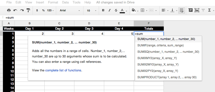
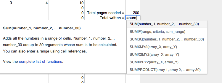
9) Enter “=SUM” into the cell. As you type, several autofill options should appear. Any time that you place “=” in a cell and begin to type words this will happen. The word “SUM” is a shortcut for adding the values of multiple cells together. Once SUM is selected, hit Enter.
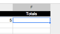
10) Your cell should look like this. Don’t click out of the cell just yet!
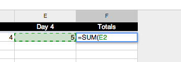
11) Click on cell E2. It should appear as an active element within equation.
12) Now, enter a comma after E2 in the equation.
14) Repeat this process with D2, C2, and B2 — inserting commas between each.
15) Finally, click Enter to complete the equation. The equation should be replaced with the total for Week 1, achieved by adding all of the daily values together within the equation in F2.
16) If you change any of the individual numbers for B2, C2, D2, or E2, the total value in F2 will reflect the change.
17) Now to copy the equation to another row. Select F2 and hit Copy on your keyboard (Ctrl+C Windows, Command+C Mac).
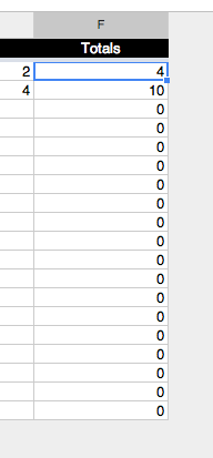
18) Select cell F3 and hit Paste on your keyboard (Ctrl+V Windows, Command+V Mac). A zero should appear.
19) The equation is transposed to calculate the sum of cells B3, C3, D3, and E3. If you enter values in those cells, the resulting total will appear in cell F3.
20) Copy/Paste the equation from F4 to F20.
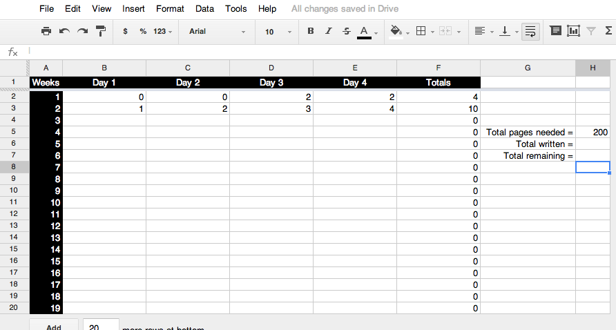
21) Now you can calculate an array of numbers. Imagine that this spreadsheet will help you to track the amount of time needed to produce a 200-page comic book. By adding two additional columns, G and H, you can estimate your grand totals. In column G, label cells G5-G7 as “Total pages needed”, “Total written”, and “Total remaining”, respectively. Enter 200 in cell H5, because that will be the ultimate length of the comic.
22) Click cell H6 and select the SUM equation from the autofill suggestions.
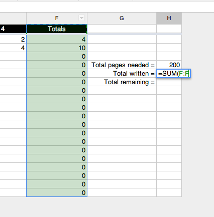
23) Hit Enter and this time, instead of clicking a single cell you will be selecting a whole column. Without leaving the equation, click “F” at the top of column F. This will select the entire column and the value “F:F” will appear in in H6.
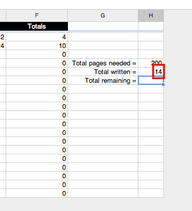
24) Hit Enter to close the equation. The total sum of column F should appear (14, if you’ve been following this example).
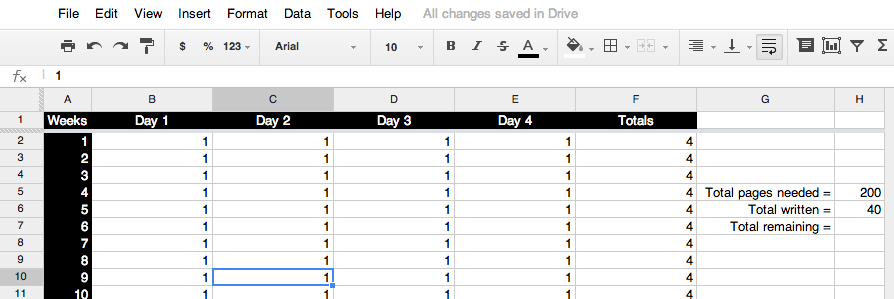
25) Now that we’ve calculated what’s been written, the next step will help us plan to hit the goal of completing 200 pages. Let’s say you have ten weeks, but feel that you can only write one page per day. Enter “1” in each of the cells in the chart. As the “Total written” value shows, that works out to a maximum of 40 pages in ten weeks.
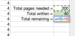
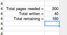
26) In order to calculate the discrepancy let’s add another equation, this time in cell H7. Enter “=” and select “=H5-H6” (Total pages needed – Total written).
27) The number of remaining pages should now appear in cell H7. (In the example, that number is 160).
28) Refer to this “Total remaining” value as you adjust the schedule. The target number of 200 will not change, nor will the number of weeks. Within that, you will need to adjust your values in terms of the number of pages written per day. The example below offers one solution for determining a production rate that will hit the goal.
Multiply & Divide
If you need to multiply or divide numbers within a cell, use the following equations:
Multiply is “=value*value”.
Divide is “=value/value”.
makingcomics.com










That was great. Although I used Numbers to make my spread sheet. Now is this how you calculate you own page count? How what is an example of deadlines? And do you use multiple columns a rows for different projects?
For page counts I generally am flexible – especially in the scripting and thumbnailing pages because the page count can change considerably between the two stages. When I go to pencil and ink I like to be locked in to a final count.
What I would do, to keep track of multiple projects, is have tabs to different spreadsheets for each. In spreadsheet, at the bottom of the page, there are tabs where you can have multiple projects within. I will have to add that to the modification section of the “Yurick Method” tutorial.
Thanks Patrick! That would be great!